Fundamentals of Antenna Arrays

To go along with this note, there are slides (PDF) and a GitHub repository with MATLAB examples that can be used to experiment with antenna arrays.

Antenna Arrays in the Real World

Antennas can be found all around us in this modern age of wireless connectivty. Wireless communication systems like 5G, Wi-Fi, Bluetooth, and satellite television/internet make use of antennas to communicate information wirelessly. Radar systems also use antennas to transmit and receive signals in order to sense the surrounding environment or detect specific objects or gestures. Radio astronomy also employs antennas to study signals that originate from stars and galaxies in deep space. All of these applications make use of antennas and in fact often make use of multiple antennas—called antenna arrays—to better achieve their communications or sensing objectives.

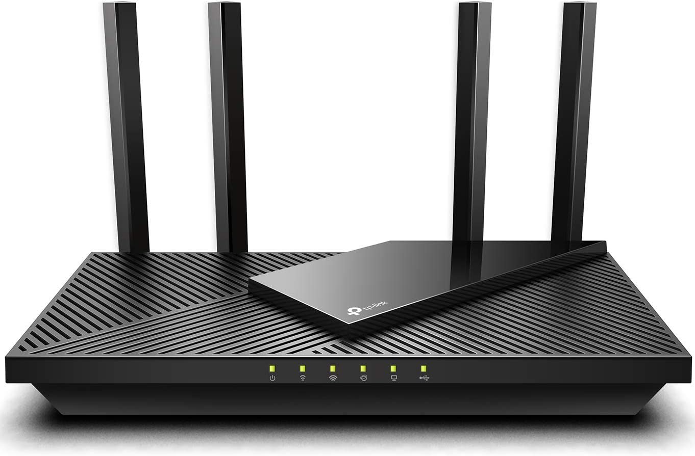
Wi-Fi

   

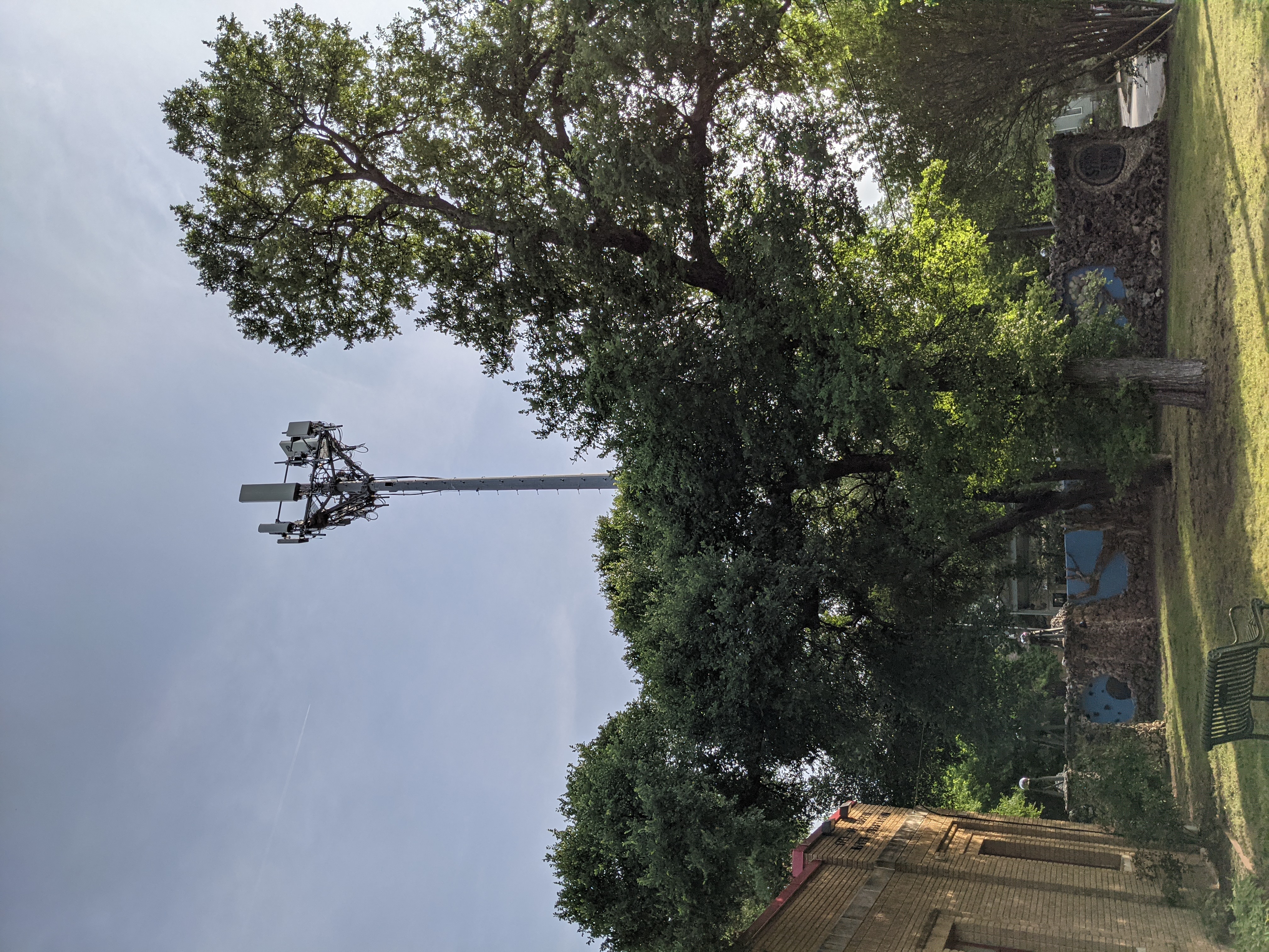
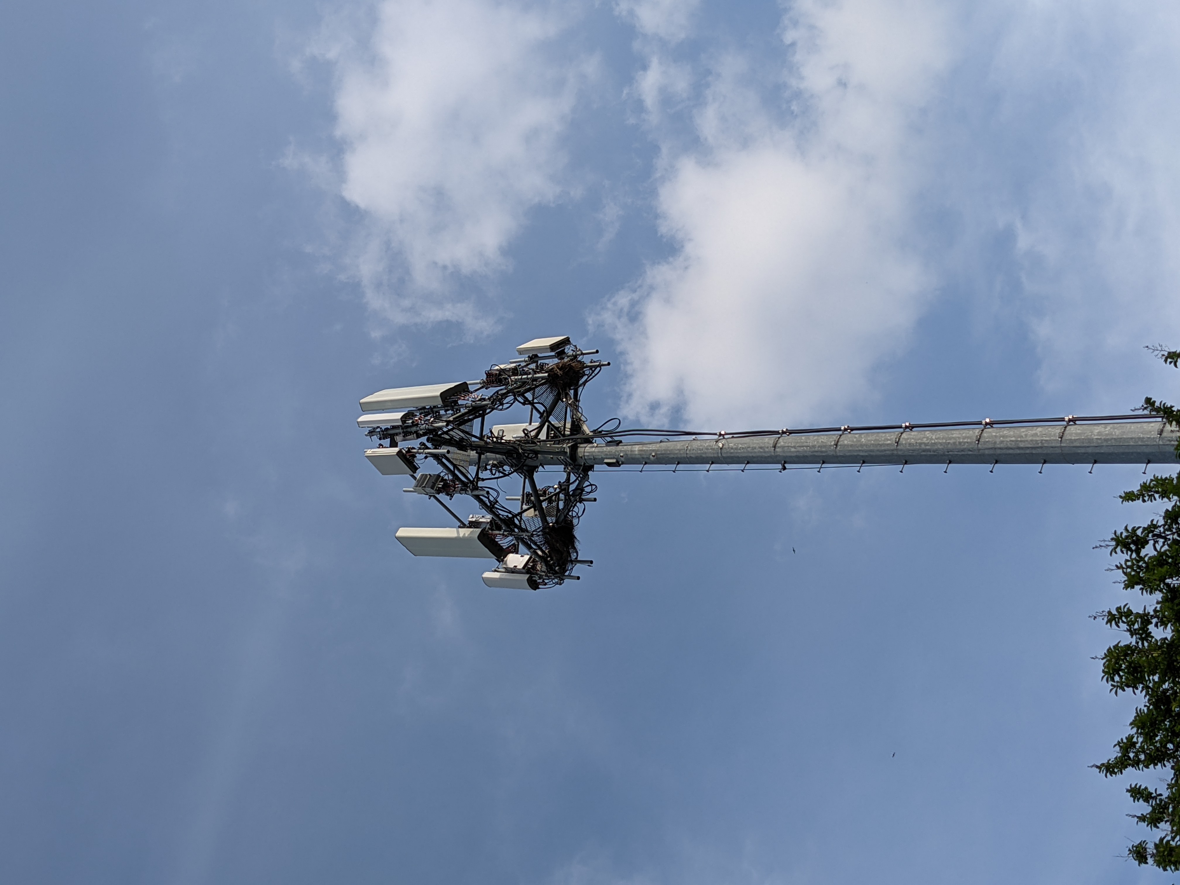
Cellular Communications

   

   

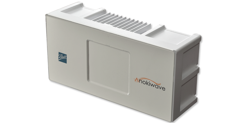
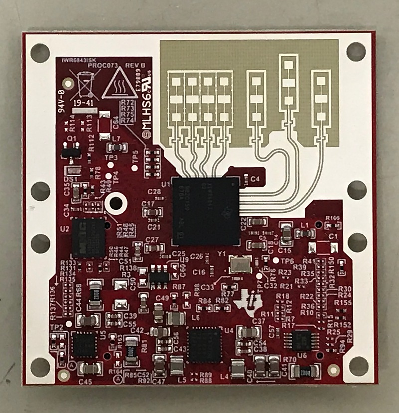
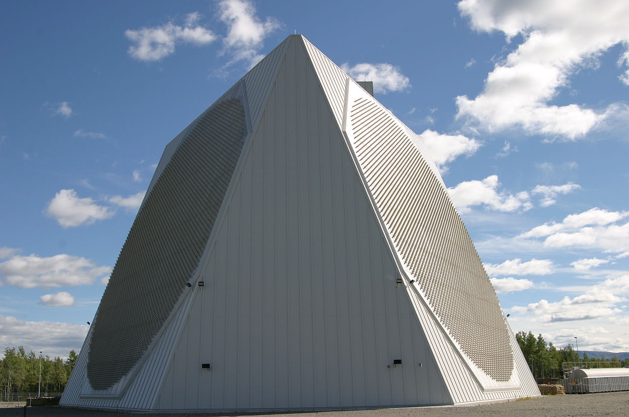
Radar

   

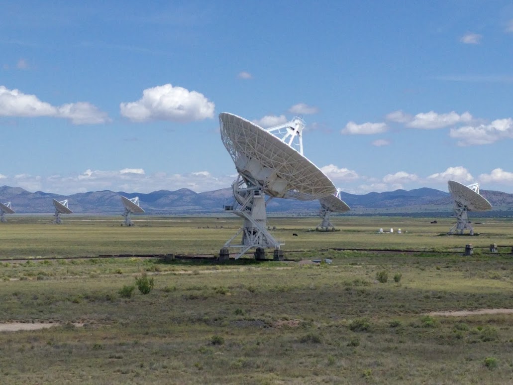
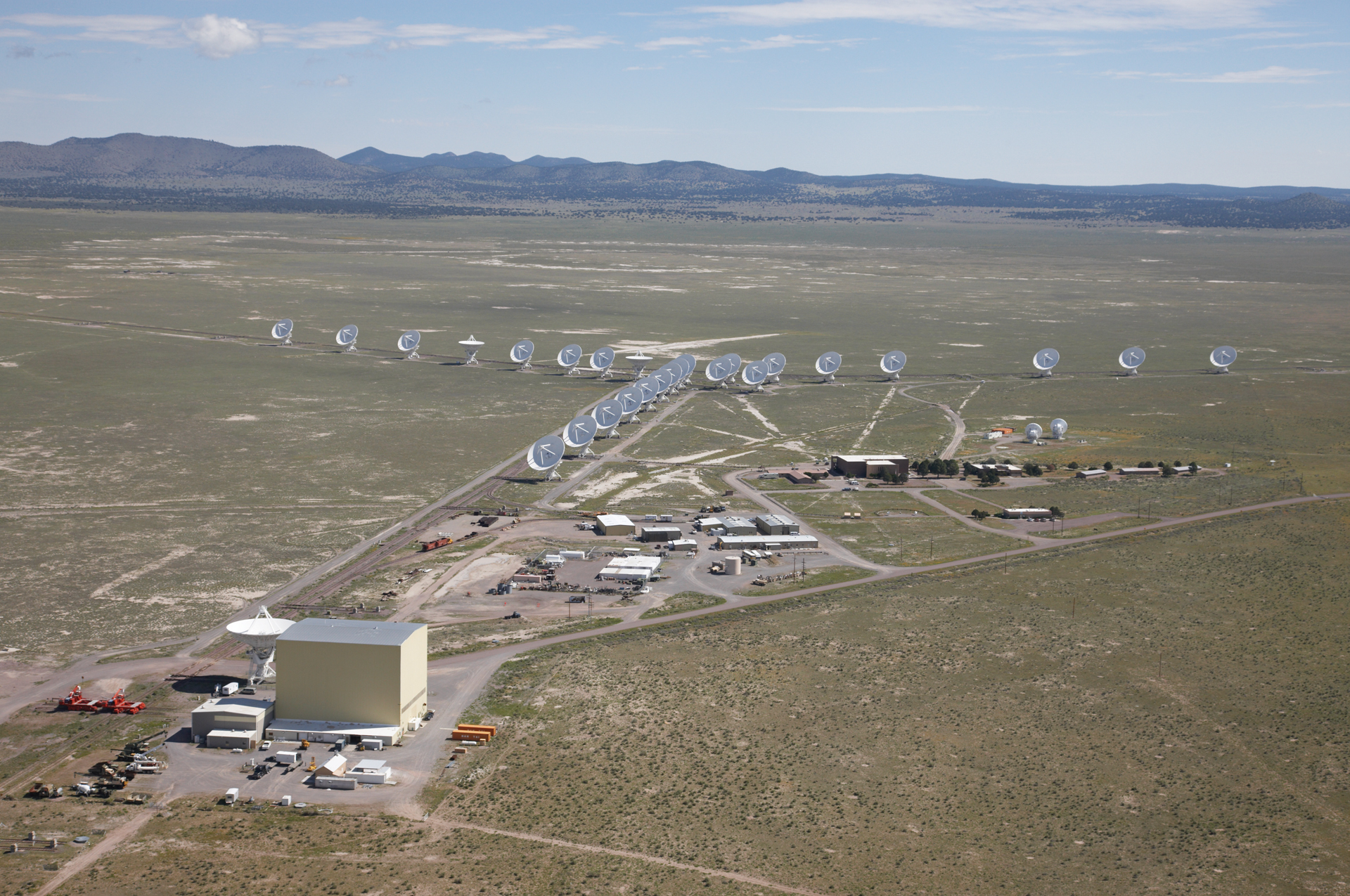
Radio Astronomy

   

What is an Antenna?

A wireless communication device—or transceiver—is equipped with one or more antennas to communicate over a wireless medium using electromagnetic waves. An antenna can be thought of as an entity that converts electrical signals to electromagnetic waves, as illustrated below. Antennas are often passive pieces of hardware (think of just a piece of metal with just the right shape), meaning they don’t require any input power. Rather, their physical properties allow them to resonate when they are fed (input) with electrical signals at just the right frequency. In other words, this resonant frequency depends on the physical characteristics of the antenna (e.g., its size, shape, and material). In general, larger antennas resonate at lower frequencies.

In addition to radiating electromagnetic waves, antennas can also be used for receiving such. When an electromagnetic wave strikes an antenna, the antenna will generate an electrical current, assuming the electromagnetic wave is at—or close to—its resonant frequency. In other words, antennas can be used for both transmission and reception of wireless signals, and in fact, antennas exhibit transmit-receive reciprocity, which means that many of their properties are the same whether the antenna is used for transmission or reception.

Antenna theory is a rich subject of its own, and this note naturally cannot cover all the details of precisely how antennas work. As such, we direct interested readers to Constantine Balanis’s textbook Antenna Theory: Analysis and Design for comprehensive coverage of the subject.

Electromagnetic Waves

As was done with antennas, we now overview necessary background on electromagnetic waves, with the understanding that more details can be found elsewhere. An electromagnetic wave propagating at some frequency $f$—either radiated or received by an antenna—can be expressed as a function of time $t$ by the sinusoid $y(t) = \sin(2\pi f t)$, as illustrated below.

For every second that passes in time, the wave completes $f$ cycles (oscillations); hence, $f$ has units of cycles/second, more commonly referred to as Hertz (Hz). Inverting the frequency $f$ of the wave, we obtain its period $1/f$, which is the time consumed when completing one cycle and has units of seconds per cycle.

Electromagnetic waves can be thought of as functions of time as described thus far, but they can also be thought of equivalently as functions of space, since as time passes, the signal propagates across space. As illustrated below, when rewriting the time axis as a spatial axis, it becomes clear that the wavelength $\lambda$ is the distance traveled when completing one cycle. The period and the wavelength can therefore be thought of as analogous quantities in the time and space domains, respectively.

To summarize the key characteristics of an electromagnetic wave concisely:

• the frequency $f$ is the number of cycles (oscillations) the wave completes in one second
• the period $1/f$ is the time consumed (in seconds) when completing one cycle
• the wavelength $\lambda$ is the distance traveled (in meters) when completing one cycle.

Electromagnetic waves propagate at the speed of light, $\mathrm{c} \approx 3 \times 10^8$ meters/sec. (On Earth, they actually travel a little slower.) Breaking down the units of wavelength $\lambda$ (meters per cycle) and frequency $f$ (cycles per second), we obtain the following relationship.

$$\underbrace{\mathrm{c}}_{\textsf{meters/sec}} = \underbrace{\lambda}_{\textsf{meters/cycle}} \cdot \underbrace{f}_{\textsf{cycles/sec}}$$

From this equation, along with our discussions prior, it becomes clear that wavelength shrinks as frequency increases. This is also illustrated below for two sinusoids, one with double the frequency of the other.

Plane Wave Assumption

An idealized antenna can be thought of as one which is infinitesimally small and radiates electromagnetic waves equally in all directions, or spherically. This concept of a so-called isotropic antenna does not truly exist in the real world but is nonetheless a useful tool in analyzing antennas.

Consider a transmitter radiating energy with an isotropic antenna, as illustrated in the animated figure below. Electromagnetic waves radiate outward from the antenna in a spherical fashion, depicted as circles here in this 2-D illustration. This can be thought of as similar to dropping a pebble in a still pond; ripples propagate outward in all directions from the point where the pebble struck the water, getting larger as they ripple outward.

   

Wavefronts Appear Planar Far from an Antenna

Suppose there are two points separated from one another by some small distance $D$. Referencing the figure below, consider the case when the two points are close to the transmitter. As an electromagnetic wave propagates out spherically from the transmitter, a spherical wavefront strikes the two points. In other words, the wave propagating over the intersection of these points appears spherical.

Slightly further from the transmitter, these two points see a slightly less spherical wavefront. Given their fixed separation $D$, the further from the transmitter, the less spherical the wavefront appears from their perspective. Far from the transmitter, the wave striking these two points appears to have a planar wavefront. This is much like how the Earth appears flat over small distances on its surface due to its large radius.

Rayleigh Distance (Far-Field Boundary)

The distance at which the spherical wavefront begins to appear as a planar wavefront is called the Rayleigh distance, often also called the Fraunhofer distance or the far-field distance/boundary.

From the perspective of an antenna whose largest dimension is $D$, the Rayleigh distance can be written as

$$\mathsf{Rayleigh~distance} = 2 D^2 / \lambda$$

where $\lambda$ is the wavelength, as usual. Notice that the Rayleigh distance increases with smaller wavelength $\lambda$ and with larger dimension $D$. The Rayleigh distance here is derived by finding the distance at which the phase profile of a wave differs by no more than $\pi/8$ radians over a distance $D$; please refer to other texts for this derivation.

Put simply, waves radiated by an isotropic antenna impinging a non-isotropic antenna with largest dimension $D$ appear approximately planar beyond the Rayleigh distance (or far-field boundary). Thanks to transmit-receive reciprocity of antennas, the Rayleigh distance also corresponds to the distance beyond which the transmitted radiation pattern of a non-isotropic antenna is no longer a function of distance; this concept of far-field in the context of transmission involves greater explanation involving electromagnetic theory, however. As we will see in the rest of this note, the far-field condition is at the root of many concepts in array signal processing and in antenna theory, in general. Conceptually, this means that it is often assumed that a transmitter and receiver are distant enough to be in the far-field of one another. In most conventional applications in wireless communications, the Rayleigh distance is on the order of centimeters or meters, meaning it is often safe to assume far-field conditions.

In general, the definition of Rayleigh distance and far-field conditions have deeper justifications tied to electromagnetic wave theory, but this simple example considering two neighboring points is also a valid interpretation of the far-field. It is important to note that electromagnetic coupling effects can manfiest when considering points extremely close to an antenna; these conditions are out of the scope of this note, however.

An Array of Two Antennas in the Far-Field

Consider two antennas close to one another, separated by some distance $d$, as illustrated below. Suppose a distant isotropic antenna—located in the far-field—radiates energy, which then impinges these two antennas. Under these far-field conditions, the radiated energy strikes the two antennas as a plane wave. When the alignment—or intersection—of these two antennas is perpendicular to the plane wave’s direction of propagation, the plane wave strikes the two antennas simultaneously.

Plane Wave from $\theta$

Now, consider the animated illustration below, which shows the case when the plane wave’s dierction of propagation $\theta$ is not perpendicular to the alignment of the antennas. As the wave propagates to the antennas, it first strikes antenna 0. Then, the wave must propagate an additional $r$ meters before reaching antenna 1.

As a result, the signal received at antenna 1 is a delayed version of the signal received by antenna 0. This time difference leads to a phase difference, as illustrated below.

To quantify this phase difference caused by propagating a distance $r$, we can employ the wave number of an electromagnetic wave. The wave number is the rate at which phase changes as a function of distance and can in fact be defined straightforwardly with tools we already have. We know a wave completes one cycle ($2\pi$ radians) every wavelength $\lambda$ that it propagates. This ratio is the wave number and has units of radians/meter.

$$\mathsf{wave~number} \ = \underbrace{\frac{2\pi}{\lambda}}_{\textsf{radians/meter}}$$

Using this, the phase difference between the signals received by the two antennas is simply

$$\underbrace{\frac{2\pi}{\lambda}}_{\textsf{radians/meter}} \cdot \underbrace{r}_{\textsf{meters}},$$

which will have units of radians. Let us now derive $r$ as a function of $\theta$ and the antenna separation $d$.

Using the geometry above, we can see that the distance $r$ is

$$r = d \sin \theta.$$

Thus, the phase difference of the signal at antenna 1 relative to that at antenna 0 is

$$\frac{2\pi}{\lambda} \cdot d \sin \theta.$$

As $\theta$ increases (the wave is less perpendicular to the antennas’ alignment), antenna 1 will see a greater relative phase shift. This phase shift can be expressed as a multiplicative term using complex exponentials (i.e., $\mathrm{e}^{\mathrm{j}\phi}$).

Let $y_0(t)$ and $y_1(t)$ be the complex signals received by antenna 0 and antenna 1, respectively. These two received signals can be related as

$$\underbrace{y_1(t)}_{\textsf{signal 1}} = \underbrace{y_0(t)}_{\textsf{signal 0}} \cdot \underbrace{\exp\left(-\mathrm{j} \cdot \frac{2\pi}{\lambda} \cdot d \sin\theta\right)}_{\textsf{phase shift at antenna 1}},$$

where $\mathrm{j}^2 = -1$ is the imaginary unit. The signal reaching antenna 1 is a phase-shifted version of the signal reaching antenna 0. Here, $-\mathrm{j}$ is used because antenna 1 sees a delayed version of the signal at antenna $0$, so the phase shift is negative, as depicted two figures above.

A Linear Array of $N$ Antennas

The results derived for two antennas can be generalized straightforwardly to uniform linear antenna arrays of $N$ elements. For clarity, let’s break down what the term “$N$-element uniform linear antenna array” means:

• $N$-element: $N$ individual antennas
• uniform: constant spacing $d$ between antennas
• linear: antennas are arranged along a line
• antenna array: multiple antennas.

A Linear Array of 3 Antennas

Let’s first look at a uniform linear antenna array of three antennas, as illustrated below.

Notice that $r_1$ is the same as $r = d\sin\theta$ that was previously derived. With simple geometry, we can see that

$$r_1 = d \sin \theta, \qquad r_2 = 2 \cdot d \sin \theta .$$

This leads to the following relationships, where $y_i(t)$ is the signal received by the $i$-th antenna.

$$\begin{aligned} y_1(t) &= y_0(t) \cdot \underbrace{\exp\left(-\mathrm{j} \cdot \frac{2\pi}{\lambda} \cdot d \sin\theta\right)}_{\textsf{phase shift at antenna 1}} \\ y_2(t) &= y_0(t) \cdot \underbrace{\exp\left(-\mathrm{j} \cdot \frac{2\pi}{\lambda} \cdot 2 \cdot d \sin\theta\right)}_{\textsf{phase shift at antenna 2}} \end{aligned}$$

A Linear Array of $N$ Antennas

We can generalize this 3-element uniform linear array to an $N$-element linear array as follows. Consider the uniform linear array of $N$ antenna elements, each separated by $d$ meters from one another.

The signal at the $i$-th antenna can be related to the signal at the $0$-th antenna as

$$\underbrace{y_i(t)}_{\textsf{signal}\ i} = \underbrace{y_0(t)}_{\textsf{signal 0}} \cdot \underbrace{\exp\left(-\mathrm{j} \cdot \frac{2\pi}{\lambda} \cdot i \cdot d \sin\theta\right)}_{\textsf{phase shift at antenna}\ i}.$$

Array Response

We can denote the phase shift at the $i$-th antenna induced by a plane wave from $\theta$ as

$$a_i(\theta) \triangleq \exp\left(-\mathrm{j} \cdot \frac{2\pi}{\lambda} \cdot i \cdot d \sin\theta\right).$$

This quantity is often called the response of antenna $i$ in the direction $\theta$.

Collecting the response at each antenna into a vector populates the array repsonse vector in the direction $\theta$.

$$\begin{aligned} \mathbf{a}(\theta) &\triangleq \begin{bmatrix} a_0(\theta) \\ a_1(\theta) \\ a_2(\theta) \\ \vdots \\ a_{N-1}(\theta) \end{bmatrix}\\ &= \begin{bmatrix} \exp\left(-\mathrm{j} \cdot \frac{2\pi}{\lambda} \cdot {0} \cdot d \sin\theta\right) \\ \exp\left(-\mathrm{j} \cdot \frac{2\pi}{\lambda} \cdot {1} \cdot d \sin\theta\right) \\ \exp\left(-\mathrm{j} \cdot \frac{2\pi}{\lambda} \cdot {2} \cdot d \sin\theta\right) \\ \vdots \\ \exp\left(-\mathrm{j} \cdot \frac{2\pi}{\lambda} \cdot (N-1) \cdot d \sin\theta\right) \\ \end{bmatrix} \end{aligned}$$

The array response vector depends on the array geometry, meaning the above expression only holds for uniform linear arrays.

An Arbitrary Array of $N$ Antennas

We now look at how to generalize the array response for arrays with arbitrary geometries. In other words, we examine how to write the array response for arrays whose elements are not arranged in a line. For example, consider the two arrays whose antenna elements are shown below.

   

Each array contains $N=16$ antenna elements. On the left, antenna elements are arranged in a planar fashion (a 2-D grid) with uniform spacing. This is referred to as a uniform planar array. The array on the right, on the other hand, has elements randomly arranged. We will look at the general form of the array response in order write it for any antenna array.

3-D Coordinate System

To do so, let’s first formally define a 3-D coordinate system. The $x$, $y$, and $z$ axes are shown as below, along with azimuth $\theta$ and elevation $\phi$. Here, azimuth $\theta$ ranges from $-\pi$ to $\pi$ radians and elevation $\phi$ ranges from $-\pi/2$ to $\pi/2$ radians.

For intuition, imagine an array centered at the origin of this coordinate system facing outward along the $y$ axis. From the array’s perspective, rightward is an increase in azimuth $\theta$ and leftward is a decrease in azimuth $\theta$. Upward is an increase in elevation $\phi$ and downward is a decrease in elevation $\phi$. Outward along the $y$ axis corresponds to $\theta = \phi = 0^\circ$. Formally, the $x$, $y$, and $z$ components of a unit vector in the direction $(\theta,\phi)$ are

$$\begin{aligned} x &= \sin\theta \cdot \cos\phi \\ y &= \cos\theta \cdot \cos\phi \\ z &= \sin \phi \end{aligned}$$

Generalized Array Response

Using the coordinate system above, suppose the $i$-th antenna an array is located at some arbitrary $(x_i,y_i,z_i)$ in 3-D space. The relative phase shift experienced by the $i$-th antenna can then be written as

$$a_i(\theta,\phi) \triangleq \exp\left(\mathrm{j} \cdot \frac{2\pi}{\lambda} \cdot \left(x_i \sin\theta \cos\phi + y_i \cos\theta \cos\phi + z_i \sin\phi\right)\right).$$

Conceptually, this expression can be thought of as decomposing the incident plane wave into orthogonal components in the $x$, $y$, and $z$ dimensions via superposition; combining these three contributions leads to the effective response as written above. Collecting these into the array response vector, we have

$$\mathbf{a}(\theta,\phi) \triangleq \begin{bmatrix} a_0(\theta,\phi) \\ a_1(\theta,\phi) \\ \vdots \\ a_{N-1}(\theta,\phi) \end{bmatrix}$$

where $N$ is the number of antenna elements.

Beamforming

Thus far, we have provided a fairly thorough examination of an array’s response when impinged by a plane wave originating from some direction $(\theta,\phi)$. What can we do with this knowledge? How exactly are multiple antennas used by Wi-Fi, 5G, radar, and radio astronomy?

Put simply, by knowing the array response of an antenna array, we can use this to our advantage in a variety of ways, such as to:

• focus transmitted signals in a particular direction (e.g., to transmit toward a particular user)
• focus received signals in a particular direction (e.g., to receive from a particular user)
• sense a particular area using radar
• observe signals originating from a distant galaxy in deep space

At the root of many of these applications is what is called beamforming. Beamforming is often used to focus either transmitted or received energy in a particular direction $(\theta,\phi)$. This is achieved by applying a complex weight to the transmitted/recevied signal at each antenna. These so-called beamforming weights are often based on knowledge of the array response in the direction of interest $(\theta,\phi)$.

   

Receive Beamforming

Let’s consider the case of using beamforming to receive in a particular direction. Consider the figure below depicting an $N$-element array with some beamforming weights $\mathbf{w}$ applied. For some incident wave propagating from the direction $(\theta,\phi)$, the array will experience some response (phase shift) at each of its $N$ antennas. This populates the array response $\mathbf{a}(\theta,\phi)$.

Beamforming weights can be applied at each antenna as illustrated above, where $w_i$ is the complex weight applied to the $i$-th antenna. In other words, the received signal at the $i$-th antenna is multiplied by some complex value $w_i$. The received signals are combined by summing them together. This weighting and subsequent combining leads to a so-called beamforming gain $g(\theta,\phi)$.

Mathematically, this process of beamforming can be written as follows. Let $y_0(t)$ be the received signal striking the $0$-th antenna. The output signal after receive beamforming can be written as

$$\begin{aligned} \sum_{i=0}^{N-1} w_i \cdot y_i(t) % &= \sum_{i=0}^{N-1} w_i \cdot a_{i}(\theta,\phi) \cdot {y_0(t)} \\ &= \sum_{i=0}^{N-1} w_i \cdot \underbrace{a_{i}(\theta,\phi) \cdot {y_0(t)}}_{y_i(t)} \\ &= {y_0(t)} \cdot \sum_{i=0}^{N-1} w_i \cdot a_{i}(\theta,\phi) \\ &= {y_0(t)} \cdot \mathbf{w}^{\mathrm{T}} \mathbf{a}(\theta,\phi) \\ &= {y_0(t)} \cdot g(\theta,\phi). \end{aligned}$$

Notice that the output signal is $y_0(t)$ amplified by some complex gain $g(\theta,\phi)$. By designing $\mathbf{w}$ to increase this gain $g(\theta,\phi)$, we can increase the received signal power, which can yield higher data rates in the context of wireless communication or can improve the sensing capability in the context of radar or radio astronomy.

Here, we have used vector notation to express the beamforming gain in some direction $(\theta,\phi)$ with beamforming weights $\mathbf{w}$ as

$$g(\theta,\phi) \triangleq \mathbf{w}^{\mathrm{T}} \mathbf{a}(\theta,\phi) = \sum_{i=0}^{N-1} w_i \cdot a_{i}(\theta,\phi)$$

where $(\cdot)^\mathrm{T}$ is the transpose operator. Note that some texts use the convention that beamforming weights are conjugated before applied; this is simply a difference of convention. If you are not yet familiar with linear algebra, you can merely ignore this notation and only consider the summations above.

The beamforming gain $g(\theta,\phi)$ is a complex number, containing some magnitude and phase. Often times, especially in communications applications, we are interested in the magnitude of $g(\theta,\phi)$, written simply as $|g(\theta,\phi)|$. This is typically because increasing the magntiude of $g(\theta,\phi)$ can increase the communication data rate, with the phase component of $g(\theta,\phi)$ being equalized after the fact.

How to Design Beamforming Weights?

Beamforming weights $\mathbf{w}$ are often designed based on one’s knowledge of the array reponse vector $\mathbf{a}(\theta,\phi)$ in the direction of interest $(\theta,\phi)$. For example, suppose we are interested in receiving toward $\theta = 30^\circ$ and $\phi = 45^\circ$. We could compute the array response vector $\mathbf{a}(30^\circ,45^\circ)$ based on the known geometry of the array elements and then construct some beamforming weights $\mathbf{w}$ based on this array response.

To illustrate this, let’s walk through a simple example using an $8$-element uniform linear array illustrated above and let’s only consider a 2-D setting with azimuth parameter $\theta$. If we set our beamforming weights to be all ones as $\mathbf{w} = \mathbf{1}$, where $w_i = 1$ for $i = 0, 1, \dots, N-1$, then what will the beamforming gain $g(\theta)$ be?

The figure below illustrates this, with the magnitude of the beamforming gain $|g(\theta)|$ on the y-axis and the azimuth direction $\theta$ on the x-axis. This plot can be interepreted as follows. With beamforming weights $\mathbf{w} = \mathbf{1}$, the array will amplify signals directly in front of the array (at $\theta \approx 0^\circ$). Signals off to the left or to the right will not see as high gain, with some being severely attenuated. This illustrates that beamforming can be interpreted as a spatial filter: some directions in space are emphasized while others are rejected.

We can more intuitively visualize beamforming by converting the figure above into a polar plot as shown below. In this plot below, the x-axis has been wrapped around in a half-circle spanning from $-90^\circ$ to $90^\circ$, with radial distance from the origin representing beamforming gain. The main lobe of high beamforming gain centered around $\theta = 0^\circ$ is often itself referred to as the beam.

Isn’t it interesting that weights $\mathbf{w} = \mathbf{1}$ emphasized signals directly in front of the array? When first introducing the concept of a plane wave, we said that plane waves originating directly in fron the array (at $\theta = 0^\circ$) impinged the antennas simultaneously, meaning there was no relative phase difference between antennas. In other words, the array response is $\mathbf{a}(0^\circ) = \mathbf{1}$, meaning the signals across the antennas are inherently aligned in phase and can therefore be summed together directly using beamforming weights $\mathbf{w} = \mathbf{1}$.

Suppose we want to steer the beam toward $\theta = 30^\circ$ instead of $0^\circ$. Let’s see how this can be achieved. A plane wave coming from $\theta = 30^\circ$ will induce an array response of $\mathbf{a}(30^\circ)$. In order to “cancel” the effects of the response at each antenna $a_i(30^\circ)$, we can set

$$w_i = a_i(30^\circ)^*$$

where $(\cdot)^*$ denotes complex conjugation. Extending this to all $N$ antenna elements, we can write

$$\mathbf{w} = \begin{bmatrix} a_0(30^\circ)^* \\ a_1(30^\circ)^* \\ \vdots \\ a_{N-1}(30^\circ)^* \end{bmatrix} = \mathrm{conj}(\mathbf{a}(30^\circ))$$

where $\mathrm{conj}(\mathbf{a})$ denotes complex conjugation of each of the elements of a vector $\mathbf{a}$. The plot below depicts the beamforming gain when using this approach.

It is clear that the beam now steers toward the desired direction of $\theta = 30^\circ$. This method is called conjugate beamforming or matched filter beamforming and will always deliver maximum gain in the desired direction. We can generalize this straightforwardly as follows to some arbitrary steering direction $(\theta,\phi)$.

$$\mathbf{w} = \begin{bmatrix} a_0(\theta,\phi)^* \\ a_1(\theta,\phi)^* \\ \vdots \\ a_{N-1}(\theta,\phi)^* \end{bmatrix} = \mathrm{conj}(\mathbf{a}(\theta,\phi)).$$

Beamforming with these weights will always yield a gain $g(\theta,\phi)=N$ in the desired direction $(\theta,\phi)$, where $N$ is the number of antenna elements in the array, as verified below. The output signal after receive beamforming can be written as

$$\begin{aligned} \sum_{i=0}^{N-1} w_i \cdot y_i(t) &= \sum_{i=0}^{N-1} w_i \cdot a_{i}(\theta,\phi) \cdot {y_0(t)} \\ &= {y_0(t)} \cdot \sum_{i=0}^{N-1} w_i \cdot a_{i}(\theta,\phi) \\ &= {y_0(t)} \cdot \sum_{i=0}^{N-1} a_{i}(\theta,\phi)^* \cdot a_{i}(\theta,\phi) \\ &= {y_0(t)} \cdot \sum_{i=0}^{N-1} 1 \\ &= {y_0(t)} \cdot N. % &= {y_0(t)} \cdot \mathbf{w}^{\mathrm{T}} \mathbf{a}(\theta,\phi) \\ % &= {y_0(t)} \cdot g(\theta,\phi). \end{aligned}$$

There are many other ways to beamform in desired directions and with other factors in mind. Conjugate beamforming as presented is a good start for readers new to array signal processing, and it is in fact used every single day in applications ranging from wireless communications to radar and beyond.

Parting Words

Multiple antennas can be used in a variety of ways beyond beamforming, such as for diversity. In addition, using multiple antennas to strategically transmit/receive signals does not always lead to highly directional beams that we have seen thus far. In settings where the wireless communication environment exhibits rich scattering, the concept of the array response and of beamforming as expressed herein is less relevant. Rather, the beams that are created are based on knowledge of the wireless channel and are not necessarily highly directional in particular directions. Perhaps this will be touched on in future notes. Interested readers can read Heath and Lozano’s textbook Foundations of MIMO Communication.

Additional Readings

Here are a few good references on antenna arrays:

• Antenna Theory: Analysis and Design by Balanis
• Foundations of MIMO Communication by Heath and Lozano
• Antenna Arrays by Prof. Sean Victor Hum